Flexinvert is a framework for the optimization of surface-atmosphere fluxes of trace species, such as greenhouse gases or aerosols. It is based on Bayesian statistics and optimizes a prior estimate of the fluxes to best fit the atmospheric observations with prescribed bounds of uncertainty. The fluxes are related to the observations through a model of atmospheric transport: in Flexinvert the Lagrangian particle dispersion model, Flexpart is used. The user should be familiar with the principles of inverse modelling as well as with running Flexpart before attempting to run Flexinvert.
Flexinvert is written in Fortran90 and has been tested using the gfortran compiler on the Linux Ubuntu operating system. To compile and run Flexinvert the following libraries are required:
- NetCDF (tested with package libnetcdff6)
- LAPACK (tested with package liblapack3)
Output from the transport model Flexpart will need to be prepared prior to running Flexinvert. For details about installing and running Flexpart, the user is referred to their website.
1. Input data and pre-processing
1.1 Atmospheric observations
Flexinvert can assimilate any type of atmospheric observation, from fixed points (e.g. stations) or moving platforms (e.g. aircraft) and from satellites. Backward trajectories (or “retro-plumes”) are calculated from the observation points to calculate the so-called source-receptor-relationships (SRRs), which are needed for the inversion.
To run Flexpart for the observations and to calculate the SRRs, there is a pre-processor, prep_flexpart (or for satellites prep_satellite), that needs to be run before running the inversion. The pre-processor reads all observations in their raw format, performs any averaging or data selection (based on the SETTINGS file), prepares the input files needed for running FLEXPART, and writes the (averaged and/or selected) observations to the file format required by the inversion.
Currently, prep_flexpart can process the following observation formats: 1) NOAA surface flasks, 2) ObsPack (versions 2.1 and 3.2), 3) WDCGG hourly data, and 4) ICOS-CP data. (Note that prep_flexpart currently only handles one format type at a time, so to use different formats, prep_flexpart will have to be run separately for each format). To read another data format will require a small modification: the best practice for this is to introduce the new format as an option in “main.f90” and to make a copy of one of the subroutines e.g. “read_basic.f90” (or whichever is closest to the new format) and modify this.
For satellites, prep_satellite sub-routines currently exist for the following retrievals: 1) TROPOMI Official XCH4, 2) TROPOMI WFMD XCH4, and 3) OCO-2 XCO2. Again, to read another retrieval type will require introducing a new subroutine based on e.g. get_tropomi.f90 and introducing the new format as an option in “main.f90”.
1.2 Atmospheric transport
The pre-processor, prep_flexpart (or for satellites prep_satellite), prepares the input files required to run Flexpart. Flexpart will calculate backwards trajectories at release (or observation) points to determine the SRRs. The SRRs for each release/observation are saved in separate files (grid_time) with the timestamp of the release/observation in the file name (for satellites it is the date and retrieval number). In addition, one file containing the sensitivity of the release/observation to the initial concentrations (grid_initial) is saved for each release/observation.
Note that for Flexinvert, Flexpart needs to be run with the COMMAND file options: LINVERSIONOUT = 1 and SURF_ONLY = 1 (these are the default settings in the pre-processor). The LINVERSIONOUT setting will write grid_time and grid_initial files for each release and, for grid_time, with a time dimension for each footprint (this is in contrast to the standard output format in which the grid_time files are written for each footprint with a time dimension for each release). The SURF_ONLY setting will write only the surface SRRs to the grid_time file, as only the surface values are required by the inversion, while the grid_initial files will contain all vertical layers (without this option all vertical layers will be written in both files, which will require more memory to store and take longer to read).
prep_flexpart by default prepares one Flexpart run for each station (or campaign) and month. The RELEASES file contains all the releases for the given month (campaign). The releases can be made either i) at regular intervals regardless of the observation timestamp (e.g. hourly) or ii) with one release per observation (or averaged observation). This is determined by the field LRELEASE in the SETTINGS file. In the case of regular releases, the frequency is set in the field RELFREQ. It possible, for example, to average the observations to e.g. 3 hourly intervals, while setting up FLEXPART releases hourly. If the FLEXPART releases are calculated at regular intervals, then the grid_time (and grid_initial) files will be selected/averaged in Flexinvert to match the observation timestamps (this is controlled by the option AVERAGE_FP in the SETTINGS_config file). Making regular (e.g. hourly) FLEXPART releases has the advantage that these can be re-used with different observation averaging intervals. Note, with this option, the averaged grid_time (and grid_initial) files are saved in NetCDF files in the directory path_flexncdf so that they don’t need to be re-averaged with each iteration of the code. If an inversion needs to be re-run, and the averaged SRRs have already been calculated, then these are read from path_flexncdf.
prep_satellite by default prepares one Flexpart run per day, which includes releases for all retrievals in that day. The retrievals can optionally be averaged onto a variable resolution grid, where the resolution is determined by the heterogeneity of the total column mixing ratios – in regions of more variability higher resolution is used vice versa. prep_flexpart prepares column equivalent SRRs for each retrieval or average of retrievals. Unlike prep_flexpart (for ground-based observations) it is not possible to average the column SRRs after having run Flexpart. For more details see the section on satellite data.
Flexinvert allows the use of nested Flexpart output domains (in SETTINGS file: LNESTED = 1). If the nested option is used, then two sets of grid_time files are written for each observation, one for the global domain (normally at lower resolution) and one for the nested domain (normally at higher resolution). In this case, the global domain files are used to calculate the so-called background mixing ratios while the nested domain files are used in the inversion step. If using this option, the nested domain for the FLEXPART runs must be the same size or larger than the domain of the inversion.
Note, if combining satellite and ground-based observations in an inversion, then the Flexpart runs for each need to have the same domain(s) and the same resolution(s).
The input files generated to run Flexpart are:
- COMMAND
- AGECLASS
- RELEASES
- OUTGRID (OUTGRID_NEST)
- pathnames
After running the pre-processor, the Flexpart jobs can be run by simply editing and executing the file “run_flexpart.sh”.
1.3 Prior flux estimates
Flexinvert requires a prior estimate of the fluxes. The fluxes are read from NetCDF files (one file for each year) and must be at the same spatial resolution as the FLEXPART grid_time files. A pre-processor, prep_fluxes, is provided to reformat the fluxes to the resolution required, this can be either by averaging or interpolating. If using a nested domain (see the section on the grid definition), then the fluxes must be provided for both the global and the nested domain with the corresponding spatial resolutions (both can be prepared by separate runs of prep_fluxes). Otherwise only the global fluxes are required.
For CO2, the inversion can optimise either NEE (net-ecosystem exchange) or NBP (net biome productivity). The difference in what is optimised lies in what is prescribed for the prior fluxes. For NEE, the prior for fossil fuel (and concrete) emissions should also include biomass burning (these are not traced separately). For NBP, the prior for fossil fuel should be only fossil fuel (and concrete) emissions, but the prior for NEE should include C-fluxes due to disturbances, such as biomass burning.
The output flux file contains the latitude and longitude dimensions (given for the mid-point of each grid-cell in degrees) and the time dimension (given in days since 1-Jan-1900).
1.4 Boundary conditions
For long-lived atmospheric species (with an atmospheric lifetime of more than a couple of weeks) the atmospheric background must be accounted for. This is because the Flexpart runs only account for the influence on the species for as long as the length of the backwards trajectory (set by AGECLASS). The background mixing ratio (or concentration) is modelled for each observation by coupling the grid_initial files to global fields of initial mixing ratios (or concentrations). The initial mixing ratio fields can be provided from prior runs of a global Eulerian model e.g. the Copernicus Atmosphere Monitoring Service (CAMS), or by an interpolation of observations representing the well-mixed troposphere from e.g. the NOAA flask sampling network. The initial mixing ratio fields need to be provided as NetCDF files.
In the case that initial mixing ratio fields cannot be provided (because there are no existing model runs or insufficient observations to interpolate) the user can modify the code to read his/her own background mixing ratio estimates. This would involve:
- modifying “init_ghg.f90” (or “init_co2.f90”) to comment-out the call to “init_cini.f90” and replacing it with a call to the user’s own sub-routine providing estimates of the background mixing ratios for each observation. This sub-routine must write the background estimate for each observation to the variable “cini” in the data structure “obs”.
- modifying “calc_conc.f90” to comment-out the lines assigning the values of “obs%bkg(i)” and “bkgerr” and setting the value of these variables to zero.
1.5 Grid definition
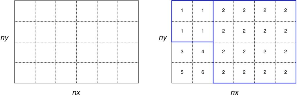
Flexinvert has the option of optimizing the state variables for each grid-cell (at the resolution of the grid_time files) or on an aggregated grid (or regions). These regions may be based on an aggregation of grid-cells using the information from the SRRs or on the user’s own definition. Using an aggregated grid has the advantage of reducing the dimension of the inversion problem, thus reducing the computation time and memory required. On the other hand, depending on the aggregation, it may increase the aggregation error.
Using an aggregated grid based on the SRRs means that there is a minimal increase in the aggregation error, as grid-cells are aggregated only where there is little information provided by the observations about the fluxes. A pre-processor, prep_regions, is provided to calculate the aggregated grid. This step requires the grid_time files (from prep_flexpart) and optionally the prior fluxes. The prep_regions pre-processor uses the same SETTINGS_files and SETTINGS_config files as used for running the inversion (namely the paths to the FLEXPART output, land-sea mask, and prior fluxes, as well as the inversion domain settings). In addition, there are user options in the SETTINGS_regions file in the same directory as prep_regions.
The grid definition is saved in NetCDF format with the filename as specified by “file_regions” defined in SETTINGS_files. This file contains a 2D matrix (lon × lat) covering the inversion domain (as defined in SETTINGS_config) at the same resolution as the grid_time files. The elements of this matrix contain a number from 1 to N where N is the total number of grid-cell aggregates (or regions). If the option USELANDUSE = true (see SETTINGS_regions) then land regions will be numbered 1 to Nland and ocean regions will be numbered -1 to –Nocean.
Note if USELANDUSE = FALSE, then no land/ocean distinction will be made in Flexinvert. The user can also provide his/her own regions definition file (instead of using prep_regions) as long as it follows the same format as the one described above. This file must cover at least the inversion domain.
1.6 Satellite data
Satellite observations can be used in Flexinvert using the total column SRRs calculated by Flexpart. Satellite observations can be used in the inversion with or without surface observations.
Retrievals can be optionally averaged (in SETTINGS avg_pixels = true) to either a predefined grid (input file specified in SETTINGS) or on a variable grid based on the variability of the total column mixing ratios:
- Predefined grid: this must be specified as a list (ascii format) of the coordinates of the lower left corners (llx and lly) of each grid cell and the grid cell resolution (in degrees), example:
| llx | lly | res |
| -180.00 | -90.00 | 6.00 |
| -174.00 | -90.00 | 6.00 |
- Variable grid: this grid is based on the standard deviation of the column mixing ratios. The minimum resolution is given by dmin, and the number of steps (including the minimum) is given by nsteps. The grid is first defined for the coarsest resolution (given as dmin × 2nsteps-1) and the retrievals are each assigned to a grid cell on this grid. The grid is refined stepwise (nsteps–1 to 1) by dividing grid cells where the standard deviation of the column mixing ratio is above cut-off. The grid is redefined each day according to the retrievals.
prep_satellite prepares two output files:
- releases_[satellite]_[spec]_YYYYMMDD.nc this file is for use in Flexpart and replaces the RELEASES file. It contains for each retrieval: horizontal location, vertical pressure layers, column averaging kernel, dry air concentration, and number of particles to release.
- retrieval_[satellite]_[spec]_ YYYYMMDD.nc this file is for use in Flexinvert and contains for each retrieval: the total column mixing ratio and its uncertainty, the prior total column mixing ratio (with and without convolution with the averaging kernel), horizontal location, and dry air concentration.
2. Running the inversion
The user settings for Flexinvert are specified in two files, SETTINGS_config and SETTINGS_files in the sub-directory “settings”. The settings files must be provided as input arguments when running Flexinvert (see “job_flexinvert.sh”).
2.1 Configuration
| Field | Description |
| run_mode | 0: forward run in which only the prior mixing ratios are modelled 1: optimization run in which the fluxes are optimized 2: random perturbation run in which random perturbations are added to the prior fluxes and observations |
| seed | this is only used for run_mode = 2 and sets the seed for the random number generation |
| datei/datef | the start and end dates for the inversion interval. These may cover multiple years but must start at the beginning a month and end at the end of a month |
| lognormal | use a lognormal distribution (true or false) |
| trunc | truncation level of eigenvalues of prior error covariance matrix (cuts at trunc × largest eigenvalue) |
| method | three options for solving the inverse problem are provided: analytic: the analytical method, which requires the full transport matrix to be stored in memory congrad: the conjugate gradient method m1qn3: the M1QN3 Quasi-Newton method |
| average_fp | (true/false) if true the grid_time and grid_initial files are averaged (or selected) to match the observation times (use this if you run prep_flexpart with LRELEASE = 0, i.e. releases at regular intervals), if false the code assumes the releases already match the observation times |
| maxiter | maximum number of iterations (only for methods “congrad” and “m1qn3”) |
| inc_ocean | (true/false) if this option is set to true fluxes over the ocean will be optimized in addition to land grid cells (note if spatial aggregation is used, then the regions must contain the distinction between land and ocean regions) |
| opt_cini | (true/false) if true, then the initial mixing ratios will be optimized in the inversion (see fields cini_lat, cini_alt, cinres) |
| spa_corr | (true/false) if this option is set to true then the error covariance matrix will contain spatial correlations between fluxes (note if large regions are used in the inversion then no spatial correlation between them should be used) |
| prior_bg | (1 = true/0 = false) this option only applies to methods “congrad” and “m1qn3” and allows the “analysis.nc” file from a previous inversion to be used as a starting point for continuing the optimization (note that this is different from the prior flux estimate, which must be the same as that used in the previous inversion). |
| restart | (1 = true/0 = false)this option can be used with methods “congrad” and “m1qn3” to continue further iterations of the inversion |
| verbose | (true/false) if true additional output is saved that can be used for debugging (note that using this option for large runs is not recommended as it will increase the computation time and produce large numbers of output files) |
| spec | currently two species types are defined: ghg: a generic greenhouse gas species co2: for inversions of CO2 and allows the fluxes to be optimised at sub-daily time steps |
| molarmass | the molar mass of the species optimized and used to convert the SRRs from mass mixing ratios to volume mixing ratios (note: the molar mass must be consistent with the mass used in the prior fluxes) |
| coeff | converts the SRRs mass mixing ratios (in units of ppt) to the unit of the observations (e.g. ppm or ppb) |
| satellite | (true/false) include satellite observations |
| ground | (true/false) include ground-based observations in the inversion (can be true if “satellite = true”) |
| coeffsat | converts the satellite total columns to units of ppbv or ppmv |
| nested | (true/false) if true uses nested output from Flexpart (grid_time_nest) over inversion domain |
| w_edge_lon | longitude of western edge of inversion domain |
| s_edge_lat | latitude of southern edge inversion domain |
| e_edge_lon | longitude of eastern edge of inversion domain |
| n_edge_lat | latitude of northern edge of inversion domain |
| xres | longitude grid resolution (must match Flexpart grid_time(_nest) resolution) |
| yres | latitude grid resolution (must match Flexpart grid_time(_nest) resolution) |
| regions | (true/false) if this option is set to true, then a spatially aggregated grid is used as defined by the file “file_regions” in SETTINGS_files |
| statres | the temporal resolution of the state vector in days (must be an integer) |
| states_hr | (for spec = co2) the sub-daily resolution of the state vector in hours (must be an integer and there must exist an integer by which this can be multiplied to give 24 hours) |
| nstep_flx | (for spec = ghg) time step of input fluxes in hours (for monthly fluxes use nstep_flx = 720) |
| nstep_nee | (for spec = co2) time step of input global NEE fluxes in hours |
| nstep_nee_reg | (for spec = co2) time step of input regional NEE fluxes in hours |
| nstep_ff | (for spec = co2) time step of input global fossil fuel (and biomass burning) emissions in hours (for monthly fluxes use nstep_ff = 720) |
| nstep_ff_reg | (for spec = co2) time step of input regional fossil fuel (and biomass burning) emissions in hours (for monthly fluxes use nstep_ff_reg = 720) |
| nstep_ocn | (for spec = co2) time step of input ocean fluxes in hours (for monthly fluxes use nstep_ocn = 720) |
| coeff_ff | (for spec = co2) coefficient to convert input global fossil fuel (and biomass burning) emissions to kg/m2/h |
| coeff_ff_reg | (for spec = co2) coefficient to convert input regional fossil fuel (and biomass burning) emissions to kg/m2/h |
| measerr | the minimum measurement uncertainty (only used if measurement uncertainty is not specified in the observation files or if it is larger than that specified) |
| cinierr | the estimated uncertainty in the initial concentration fields specified as a fraction |
| flxerr | the prior flux uncertainty specified as a fraction |
| flxerr_ll | the lower limit for the prior flux uncertainty (in the same units as the input fluxes) and is used to avoid having zero uncertainty where the prior flux estimate is zero |
| sigma_land | the spatial correlation scale length over land in km (only used if spa_corr is true) |
| sigma_ocean | the spatial correlation scale length over ocean in km (only used if spa_corr is true and ocean fluxes are optimized) |
| sigmatime | the temporal correlation scale length in days |
| globerr | an estimate of the domain total error in Tg/y and is used to scale the prior error covariance matrix (to switch scaling off set globerr = -1) |
| cini_lat | used for the optimisation of the initial mixing ratios: comma separated list of northern edges of latitude bands |
| cini_alt | used for the optimisation of the initial mixing ratios: comma separated list of upper level of vertical bands (upper most level > outheight(nzgrid) |
| cinires | used for the optimisation of the initial mixing ratios: time resolution (days) |
2.2 Monte Carlo ensembles
If the conjugate gradient method is used, the estimate of the posterior uncertainty found by the conjugate gradient algorithm gives only a poor approximation of the actual uncertainty, and for the M1QN3 method, the posterior uncertainty is not estimated at all. In these cases, Flexinvert can be used to generate a Monte Carlo ensemble of inversions, which can be used to approximate the posterior uncertainty more reliably. This requires multiple inversion runs, as one inversion equates to one member of the ensemble, with each run using “run_mode = 2″ and a different value for “seed”. The standard deviation of the posterior fluxes from the ensemble provides an estimate of the posterior uncertainty.
3. Output data
All output are saved to the directory specified by “path_output” in SETTINGS_files.
| File | Description |
| analysis.nc | the prior and posterior fluxes, flux increments and uncertainties, as 3D arrays (lon × lat × time) (for CO2, the prior fossil fuel (and biofuel) and ocean fluxes are also included) (note: if using the method “congrad” or “m1qn3” the posterior uncertainties in this file should not be used but instead calculated using a Monte Carlo ensemble) |
| analysis_nee.nc | (for spec = co2) the prior and posterior NEE fluxes and flux increments (at the same temporal resolution as the prior) as 4D arrays (lon × lat × day × hour) |
| area_box.txt | the areas of the cell aggregates (or regions) in square meters |
| correl.txt | the spatial correlation covariance matrix as a 2D array (nbox × nbox) |
| cort.txt | the temporal covariance matrix as a 2D array (ntstate × ntstate) |
| cost.txt | (M1QN3 method only) the cost at each iteration |
| evals.txt | the eigenvalues of the prior error covariance matrix for 1 time-step |
| evecs.txt | the eigenvectors of the prior error covariance matrix for 1 time-step |
| flexinvert.log | the logfile of the inversion run |
| grad_XX.txt | (congrad and M1QN3 methods only) the gradient of the cost function at iteration XX |
| hessian_evals.txt | (congrad method only) the eigenvalues of the Hessian matrix |
| hessian_evecs.txt | (congrad method only) the eigenvectors of the Hessian matrix |
| hloc_box.txt | the difference from UTC in hours for each grid cell aggregate (or region) |
| lsm_box.txt | the land-sea mask for the grid cell aggregates (or regions) |
| monitor.txt | the modelled and observed atmospheric mixing ratios (or concentrations) |
| nbox_xy.txt | the definition of the aggregated grid as a 2D array (lon × lat) |
| obsdatatype.txt | the observed and initial mixing ratios, where the initial mixing ratio is written for each component of cini_lat and cini_alt |
| obsfiles.txt | the number of observation files read (first entry) and a list of the files |
| obsread.txt | the observed mixing ratios (or concentrations) and their uncertainty for all sites and times |
| scalars_cini.txt | (only if opt_cini is true) prior and posterior scalars for the background mixing ratios and their uncertainty |
| sqcort.txt | the square root of the temporal covariance matrix as a 2D array (ntstate × ntstate) |
The modelled and observed mixing ratios are written as the following variables in monitor.txt:
| Variable | Description |
| conc | observed mixing ratio (or concentration) |
| cini | initial mixing ratio (contribution from particle termination points) |
| cinipos | optimized initial mixing ratio (contribution from particle termination points) |
| bkg | background mixing ratio (contribution from fluxes outside domain) |
| ghg | (if spec = ghg) total contribution from inside domain fluxes |
| nee | (if spec = co2) contribution from NEE fluxes |
| fff | (if spec = co2) contribution from fossil fuel (and biofuel) fluxes |
| ocn | (if spec = co2) contribution from ocean fluxes |
| prior | contribution from the prior state vector (zero ) |
| post | contribution from the posterior state vector |
| cpri | for satellite data this is the prior total column mixing ratio (otherwise zero) |
| cakpri | for satellite data this is the prior total column mixing ratio convolved with the averaging kernel (otherwise zero) |
| diff | the model-observation differences |
| error | the total error in the observation space |
The total prior and posterior modelled mixing ratios can be calculated from the monitor.txt file as follows (note that the components in parentheses are only needed for satellite observations):
For CO2:
| ypri = ycini + ybkg + ynee + yfff + yocn + yprior ( + ycpri – ycakpri) |
| ypos = ycinipos + ybkg + ynee + yfff + yocn + ypost ( + ycpri – ycakpri) |
For GHG species:
| ypri = ycini + ybkg + yghg + yprior ( + ycpri – ycakpri) |
| ypos = ycinipos + ybkg + yghg + ypost ( + ycpri – ycakpri) |
4. Quick reference guide
This section provides a quick reference guide summarizing all the steps needed to prepare and run Flexinvert.
- Prepare observations and Flexpart runs
Using the pre-processor prep_flexpart:- Compile using “make”
- Edit the SETTINGS file
- Edit the bash script: job_prep_flexpart.sh (or alternatively for slurm: sbatch_prep_flexpart.sh)
- To prepare the flexpart input files and observations, run the bash script: ./job_prep_flexpart.sh (or ./sbatch_prep_flexpart.sh)
- To run the flexpart jobs, edit run_flexpart.sh and run using ./run_flexpart.sh
- Prepare satellite observations and Flexpart runs
Using the pre-processor prep_satellite:- Compile using “make”
- Select the appropriate SETTINGS file for the satellite and edit
- Edit the bash script: sbatch_satellite.sh
- To prepare the flexpart input files and observations, run the bash script: ./sbatch_satellite.sh
- To run the flexpart jobs, edit run_flexpart.sh and run using ./run_flexpart.sh
- Prepare fluxes on the Flexpart grid
Using the pre-processor prep_fluxes:- Compile using “make”
- Edit the file FLUXES
- Edit the bash script: job_prep_flux.sh (or alternatively for slurm sbatch_prep_flux.sh)
- Run the bash script: ./job_prep_flux.sh (or ./sbatch_prep_flux.sh)
- Prepare regions definition file (optional)
Using the pre-processor prep_regions:- Compile using “make”
- Edit settings/SETTINGS_config and settings/SETTINGS_files (i.e. same settings files as used for the inversion)
- Edit SETTINGS_regions
- Edit the bash script: job_prep_regions.sh (or alternatively for slurm: sbatch_prep_regions.sh)
- Run the bash script: ./job_prep_regions.sh (or ./sbatch_prep_regions.sh)
- Run Flexinvert
- Compile using “make”
- Edit settings/SETTINGS_config and settings/SETTINGS_files
- Edit the bash script: job_flexinvert.sh (or alternatively for slurm: sbatch_flexinvert.sh)
- Run the bash script ./job_flexinvert.sh (or ./sbatch_flexinvert.sh)